Wednesday, 18 April 2018

How to use GCDkit in a batch mode II


In one of the earlier blogs, Jeff has presented my exercise showing effective use of batch mode borrowed from our joint workshop at University of Catania.  

Here I would like to carry on and show the new capabilities of GCDkit to use multiple datasets and to overplot them on a single diagram (or plate thereof).

Binary plot

# Loading and storing the 1st dataset
data(atacazo)
accessVar("atacazo")
assign1col("gray")
pokeDataset("atacazo",overwrite.warn=FALSE)

Loading and storing the 2nd dataset
data(sazava)
accessVar("sazava")

Switching back to the atacazo dataset
peekDataset("atacazo")
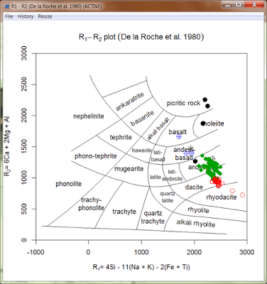
# Overplotting classification diagram
plotDiagram("TAS",F,F)
overplotDataset("sazava",pch="*",col="red",cex=2)

Spiderplot

# Overplotting on spiderplot
peekDataset("atacazo")

# Atacazo as grey field
spider(WR,"Boynton",0.1,1000,field=TRUE,fill.col=TRUE,
  shaded.col="khaki")
overplotDataset("sazava")


A plate (Harker plots)

# blatna dataset
data(blatna)
accessVar("blatna")
multiple("SiO2","MgO,CaO,Na2O,K2O")
plateXLim(c(53,70)) # Common x axis scaling
plate0YLim() # All y axes start from 0

plateCex(1.5)
plateCexLab(1.5)
plateCol("gray")

# Overplot sazava on top of it
overplotDataset("sazava",cex=2)


# Getting rid of the datasets other than the current (blatna)
purgeDatasets()

User-defined diagrams in GCDkit 5.0


Due to a popular demand, the new version of our program comes with a straightforward possibility of adding (Figaro-compatible) templates for both stand-alone binary/ternary diagrams and plates. If done correctly, they integrate seamlessly into the GCDkit system, namely into the menu 'Plots|User defined...' .

There are still some limitations, though. So far, the user-defined diagrams cannot be used for classification purposes (and hence for defining subsets, groups…).  We cannot offer language versions other than English, either.

Principle

All *.r or *.R files stored in the directory Diagrams/User , except for those whose name starts with underscore ("_"), are sourced every time the menu item 'Plots|User defined...' is invoked. Hence the list of available diagrams is always built on fly, using the function .userlist().

The ordering information and name under which it appears in the menu are integral parts of the template. For stand-alone, single Figaro plots, the crucial information is:
  • Name of function defining a diagram
  • Name of the plot: sheet$demo$template$GCDkit$plot.name
  • Sequence number of the plot in the menu: sheet$demo$template$GCDkit$plot.position

For a plate of Figaro templates:
  • Name of function defining a plate
  • Name of the whole plate: plate$plot.name
  • Sequence number of the plot in the menu: plate$plot.position 

In both cases, the file should define a single function of a name identical to (the root of) the filename.
 'Sequence number' above is any positive real number (i.e., it does not have to be an integer).

Documentation

The HTML documentation is linked to the help system automatically. However, this is only done when the *.htm file, named exactly like the function, resides in Diagrams/User/doc subdirectory.

An example

Here is an example of the Al2O3/SiO2 vs MgO/SiO2 binary plot of Paulick et al. (2006). This is done using the function Paulick provided in the file Paulick.r  of  the current GCDkit distribution.


#####################################################################
#                  Al2O3/SiO2 vs MgO/SiO2 binary plot               #
#                   Fig. 3 in Paulick et al. (2006)                 #
#  Paulick, H., Bach, W., Godard, M., De Hoog, J.C.M., Suhr, G.,    #
#  Harvey, J., 2006. Geochemistry of abyssal peridotites (Mid-      #
#  Atlantic Ridge, 15o20'N, ODP Leg 209): implications for fluid/   #
#  rock interaction in slow spreading environments. Chemical Geo-   #
#  logy, 234: 179-210.                                              #
##################################################################### 
Paulick<-function(){
    x.data<<-WR[,"Al2O3"]/WR[,"SiO2"]
    y.data<<-WR[,"MgO"]/WR[,"SiO2"]

    temp<-list(
lines1=list("lines",x=c(0,0.1),y=c(1.1,0.842),
col="darkgray", lwd=10),
GCDkit=list(
"NULL",
plot.type="binary",
plot.position=12,
plot.name="Al2O3/SiO2 - MgO/SiO2 (Paulick et al. 2006)"
)
)

temp2<-list(
text1=list("text",x=0.095,y=1.008,
text="Terrestrial Array\n(melting trend)",
col="black",adj=c(1,0.5),srt=-10),
            text2=list("text",x=0.002,y=1.15,text="Depleted",
col=plt.col[2],adj=c(0,0.5)),
text3=list("text",x=0.099,y=0.83,text="Enriched",
col=plt.col[2],adj=c(1,1))
      )

if(getOption("gcd.plot.text")) temp<-c(temp,temp2) # Text on?

sheet<<-list(
  demo=list(
fun="plot",
call=list(
xlim=c(0,0.1),ylim=c(0,1.4),
main=annotate("Al2O3/SiO2 - MgO/SiO2 plot
  (Paulick et al. 2006)"
),
col="green",bg="transparent",fg="black",
xlab=annotate("Al2O3/SiO2"),
ylab=annotate("MgO/SiO2")),
template=temp
  )
)
}  

Saturday, 14 April 2018

Version 5.0 has been just released!


On March 28, 2018 has been released a new version of GCDkit 5.0. It was developed in R 3.4.3 and code-named El Chupacabra. The most important changes are summarised below.


Towards a platform-independent version
  • It is well-known that the GCDkit has been originally designed as a Windows-only package. From the current version it is possible to install  and run it also on operation systems other than Windows,  most notably Linux or Mac OSX.  
  • So far, this concerns command-line/batch mode only. 
  • The platform-independent graphical user interface (menus, dialogue boxes...) written in Tcl/Tk language  is ready and just being tested. If you are feeling unadventurous, and work on Linux and/or Mac, please do get in touch and you can become one of the beta testers. 

New Windows installer
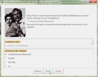
  • As we hope, we have fixed the long-standing problems with the installation of GCDkit on Windows 10, and people without administrative rights.
  • The new GUI installer, based on the Tcl/Tk  language,  is started by simply dragging the file @INSTALL.r from the temporary installation directory onto the R Console window. 
  • his file can be also located manually and loaded using the  File|Source R code...'  menu. See the download page for more details. 
  • Please note that this installer relies on a live Internet connection to download the missing packages required by the GCDkit. 


User-defined templates
  • User-defined templates for stand-alone Figaro plots or their plates. They can be uploaded into the  directory Diagrams/User and then employed for standard plotting (i.e. not classification)  purposes. This mechanism allows easy and fully automatic expansion of the plotting capabilities  of the GCDkit system. For further info, see the file @README.txt in the directory in question.
  • There are five examples of user-defined templates provided: three binary plots for discrimination of lavas from destructive plate boundaries (Pearce 1982), ternary plot for classification of A-type granites (Grebennikov 2014) and binary plot of Paulick et al. (2006) to portray the mantle peridotite fertility.  

Overplotting two or more datasets on a single diagram (or plate)
  • Functions allowing overplotting new datapoints onto standard single binary plots, ternary plots,
    spiderplots or multiple plots, including the diagram templates (overplotDataset, underplotDataset) linked to the menu system. 
  • In addition, there are functions figOverplot and figOverplotDiagram but these are meant mostly for internal use. 
  • For plotting serves a reference dataset, either real-world data (say compiled from literature) or a numeric  matrix spanning, for instance, from petrogenetic modelling.
  • See the example of overplotting the atacazo over sazava dataset on De la Roche et al. (1980) plot.
  • Very attractive feature should be the new possibility of obtaining dataset by online search of the EarthChem.org database. The search can be performed directly from the menu GCDkit|Online search EarthChem.org.  It invokes a graphical front-end, written By Oscar Laurent (ETH, Zurich) that allows to enter the desired search criteria. On Windows, it also includes a primitive, and still rather slow, possibility of selecting a polygon of interest from a map of the World. 


Further new features/important changes
  • New plugin 'disclosure' for log-transformation of compositional data.
  • New geotectonic/general purpose diagrams
    • La/Yb vs. Nb/La and La/Yb vs. Th/Nb of Hollocher et al. (2012)
    • La/10-Y/15-Nb/8 of Cabanis and Lecolle (1989)
    • Zr/Y-Th/Yb of Ross and Bedard (2009)
    • YbN vs. LaN/YbN of Martin (1986) to distinguish adakites and TTGs
    • F-M-W diagram (Ohta and Arai 2007) for chemical weathering of igneous rocks
  • calcAnomaly, a function for calculating a magnitude of any anomaly on any spiderplot, based on concentrations of selected neighbouring (not necessarily adjacent) elements.
  • Spanish translation of the classification plots (courtesy of Tomas Grijalva,  Geology Department of UNAM, Mexico).
  • New zircon saturation model of Boehnke et al. (2013).
  • New training dataset atacazo.data giving the whole-rock major- and trace-element contents,   together with Sr and Nd isotopic compositions of lavas from two volcanic complexes in Ecuador: the Atacazo and the Ninahuilca (Hidalgo 2006; Hidalgo et al. 2008).   This dataset, kindly provided by Silvana Hidalgo, is used in a worked example (chapter 25) of Janousek et al.’s book (2016).
  • Another new training dataset blatna.data from the Central Bohemian Plutonic Complex, Czech Republic  (Janousek et al. 2000, 2010). It could be, together with sazava.data already present, used to test dataset switching etc.
  • New function figFixLim() extends the scales of both axes of a binary plot automatically  if necessary to accommodate all the data points.
  • new training dataset blatna.data from the Central Bohemian Plutonic Complex, Czech Republic (Janousek et al. 2000, 2010). It could be, together with sazava.data already present, used to test   dataset switching etc.
  •  New function figFixLim()extends the scales of both axes of a binary plot automatically  if necessary to accommodate all the data points.
  • New normalization scheme of Anders and Grevesse (1989) for chondrite-normalized REE spiderplots.
  • Better behaviour of many functions in batch mode (in RTerm, Jupyter, on Linux/Mac etc.)......

  • We trust that you will find this new release useful and reasonably stable.

    Good luck, Vojtech